Formatting Sentences With Functions In Google Sheets

The PROPER function works great for names since it capitalizes the first letter of every word, but it doesn’t work for formatting sentences. What if you only want to capitalize the first letter of sentences? Formatting sentences can be done with a combination of functions. This article will show you how.

Making It Happen

Formatting sentences with functions can get a bit complicated, but once you get it, all you need to do is copy it anywhere you need.

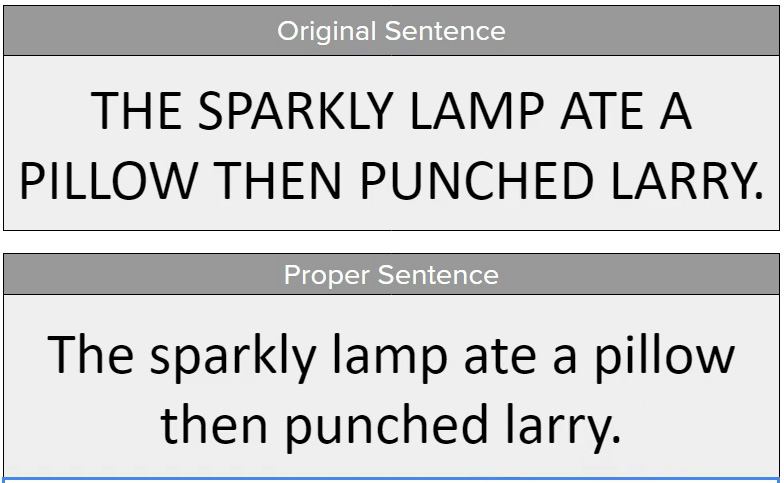
This example has been typed in all uppercase letters, but needs to be formatted properly so that only the first letter is uppercase.

Building the Function

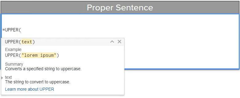
Begin with the upper function to put the first letter of the sentence in uppercase.
=UPPER(

Adding the LEFT Function

For the first value, use the LEFT function and select the cell containing the sentence to be formatted (this example uses B6). This will tell it which text to look at.
=UPPER(LEFT(B6,

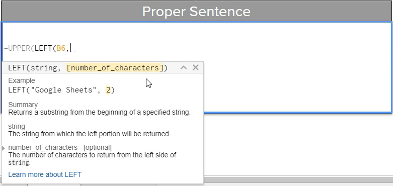
For the second value of the LEFT function, which is how many characters over it will consider, enter the number 1. This tells it to capitalize one letter from the left of the text. Then close the LEFT function and close the UPPER function, meaning you need two brackets.
=UPPER(LEFT(B6,1))

LOWER for the Next Part

Now that you’ve told it what to capitalize, you need to tell it what should be lowercase. The next step is to append this function with the ampersand symbol, telling it to add this next part.
=UPPER(LEFT(B6,1))&

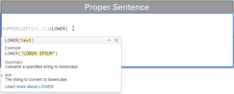
For the next part you will start with a LOWER function, and essentially do the reverse of what was just done for upper. This will tell it to lowercase everything, except the first letter.
=UPPER(LEFT(B6,1))&LOWER(

Nesting the RIGHT Function

For the first value of the LOWER function, nest in the RIGHT function. This will tell it to look at the text and begin counting characters from the right.
=UPPER(LEFT(B6,1))&LOWER(RIGHT(

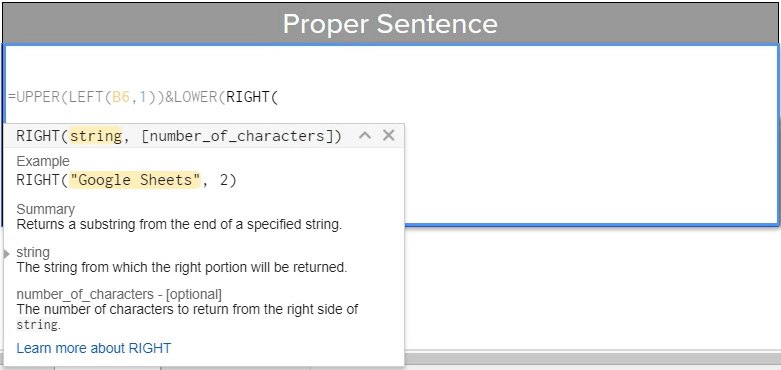
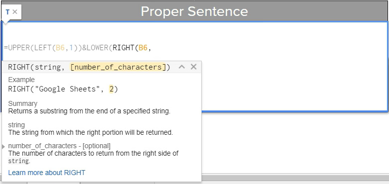
For the first value in the RIGHT function, select the text that’s being formatted (the same one that was used for LEFT). This tells it what text to look at.
=UPPER(LEFT(B6,1))&LOWER(RIGHT(B6,

Using the LEN Function

Now you need to nest one more function. For the second value of the RIGHT function, use the LEN function, which tells it the length of the string of text that’s being considered. For the LEN value, select the text again then close the LEN function.
=UPPER(LEFT(B6,1))&LOWER(RIGHT(B6,LEN(B6)

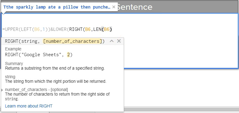
Now it’s looking at the entire length of text in that cell. Add a minus one, which tells it to look at all of the text minus the first character from the right.
=UPPER(LEFT(B6,1))&LOWER(RIGHT(B6,LEN(B6)-1

Finishing the Whole Thing

Close the RIGHT function and the LOWER function, and press Enter. You should then see the formatted result, as in the example below.
=UPPER(LEFT(B6,1))&LOWER(RIGHT(B6,LEN(B6)-1))

What Do You Do With This?

Once you have the formula down, all you need to do is copy it for all the rest of the sentences that need to be modified, as in the below example.

You can copy and paste the function from here if you’d like. However, I do recommend trying it on your own, so that you really understand how it works.

Watch the Video

Watch the video for capitalizing sentences to see it in action.

I hope you found this article to be helpful. Comment and let me know what you think.

Learn more about functions in Google Sheets with Udemy course, Understanding and Building Functions.