Freezing Rows in Google Sheets
![Freeze rows and columns in Google Sheiets](https://i0.wp.com/digitalegghead.com/wp-content/uploads/2019/01/DE-YouTube-Thumbnail-Sheets-Freeze-Rows.jpg?resize=1024%2C576&ssl=1)
You can freeze as many rows or columns as you want in Google Sheets. Here’s how:
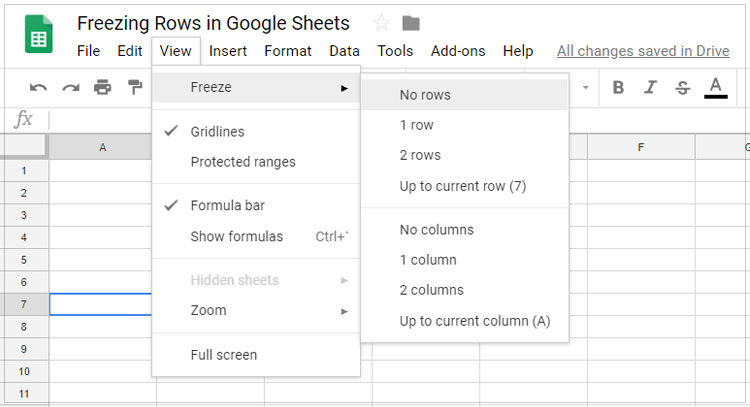
In the menu, click on: View > Freeze
Choose one of the options for either rows or columns:
- 1 row
- 2 rows
- Up to current row
![Freezing rows in Google Sheets menu selection](https://i0.wp.com/digitalegghead.com/wp-content/uploads/2019/01/DE-Article-Image-Google-Sheets-Freeze-Rows-01.jpg?resize=750%2C481&ssl=1)
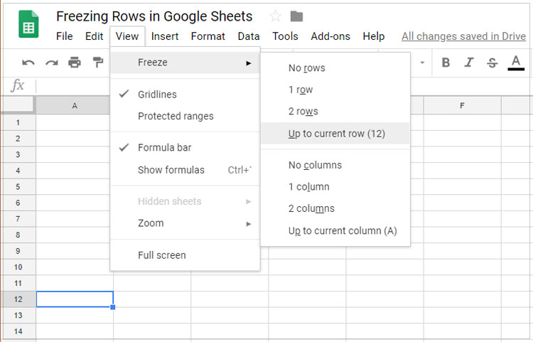
Choosing ‘up to current row/column’ will freeze to the row or column that you currently have highlighted.
Unfreezing Rows or Columns
To unfreeze the rows or columns simply follow the same steps and click on either “No rows” or “No columns”.
![Google Sheets unfreeze rows and columns](https://i0.wp.com/digitalegghead.com/wp-content/uploads/2019/01/DE-Article-Image-Google-Sheets-Freeze-Rows-02.jpg?resize=750%2C407&ssl=1)