Google Sheets Custom Date Format

Dates can be displayed in many formats in your spreadsheet. This article will show you how to set up a custom date format to your liking.

Adding Dates to a Spreadsheet

When you first enter a date into your spreadsheet, Google Sheets will usually recognize it as a date and format it accordingly. Unless you’ve already applied a different format to that cell. This is great, if you want it to be in that particular date format. However, sometimes you may want the dates to show text for the month or day, or display all four numbers for the year. Those are just a couple of examples, but there are lots of ways to format a date.

Changing the Date Format

You can change the date format from the “Format” menu under Number > More Formats > More date and time formats.

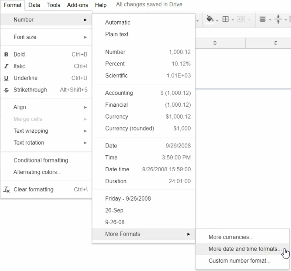
That’s a long path, but it will take you to the window where you can set up custom formats. At the top of the window, there is a field that shows the current format. Which by default is Month/Day/Year. The parentheses show an example of what the output will look like. For example, the month and say sections will be displayed as a single digit without a zero in front and the year will display with two digits.

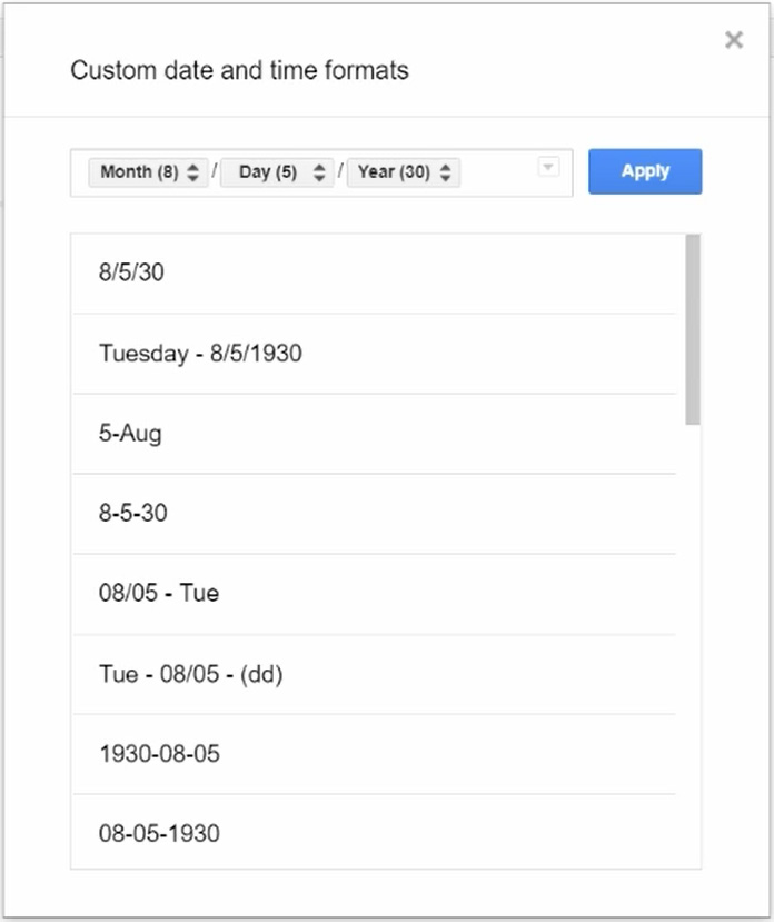
Between each portion of the date, notice that there is a slash. This tells Sheets that you want a slash do display in those spaces. This can be anything you want it to be. For example, the slashes could be replaced with hyphens.

When you click on apply, the date will update with hyphens between the numbers.

Below the top custom date field, there is a good selection of pre-configured date and time formats.

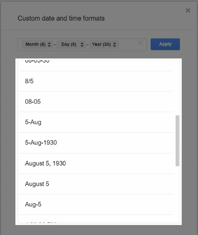
Formats that you have previously set up will also show up here. You can simply select one of these and click on Apply if it suits your needs.

 

Creating a Custom Date Format

This gives you a lot of flexibility for how you display your dates. Now, what if you don’t see a format you want? In this case, you can create your own.

Clear out the current format by clicking into the field and pressing the Backspace key to remove the different elements. To add a piece of the date, click on the little down arrow on the right side of the field.

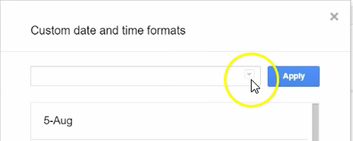
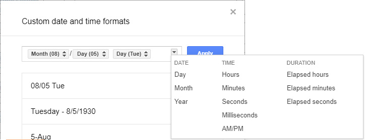
It’s not very noticeable, but it’s there. This is where you can select the elements that you need. To change how an element looks, click on the gray box to see some options.

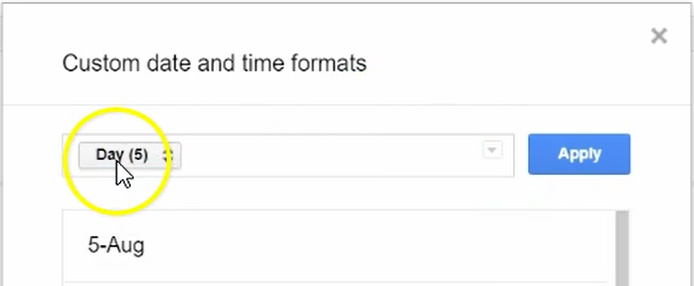
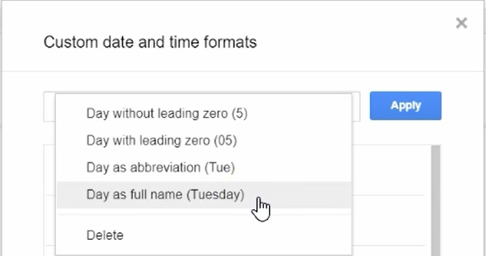
In this manner, you can add all of the elements you need and have them display how you would like.

Example Custom Date Format

Here is an example of a custom format.

 

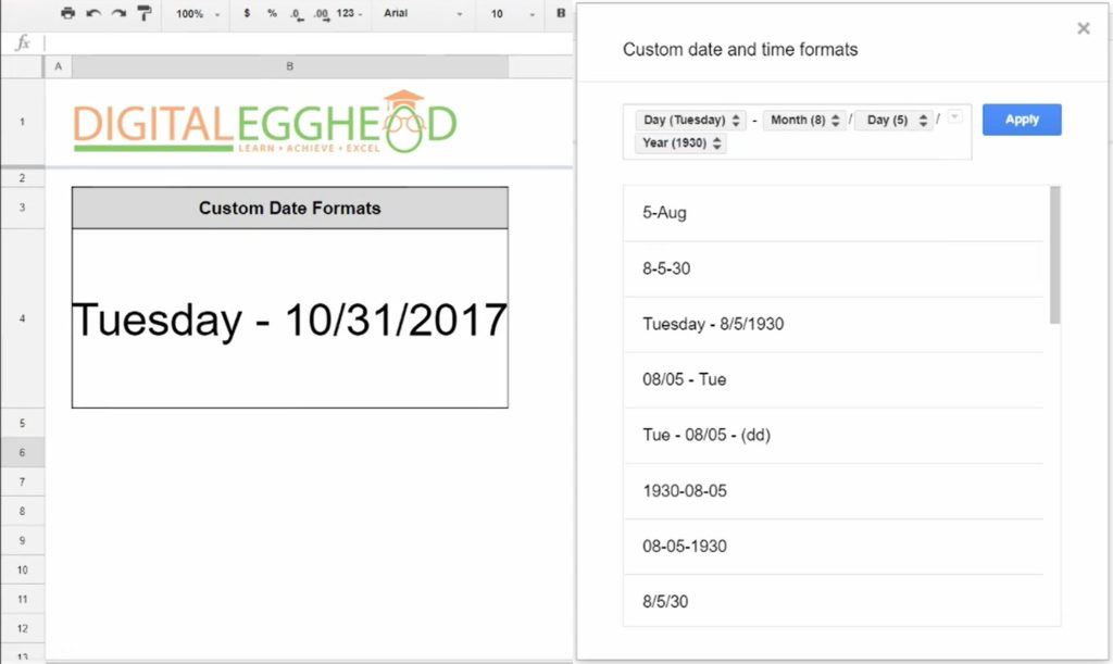
There’s a lot of power for customization here. Play around with this in your own spreadsheet to see what kind of date formats you can come up with.

Watch the Video

Watch the video to better learn how to create a custom date format in Sheets.

I hope you found this article to be helpful. Comment and let me know what you think.

Learn more about Google’s amazing office apps with the Google Cloud Productivity course on Udemy.