Conditional Date Formatting in Sheets

I’ve had this question come up a lot over time. How do I make a cell change to red or green based on the date? Fortunately, conditional date formatting is pretty easy with Google Sheets.

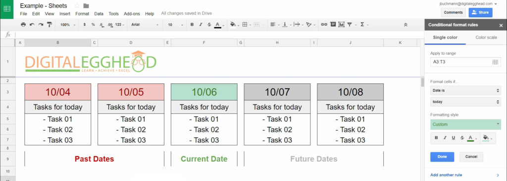
The example below shows a list of days, and tasks for each day. Right now they’re all grey. We want to have the date show as red for past dates, green for the current date, and gray for future dates.

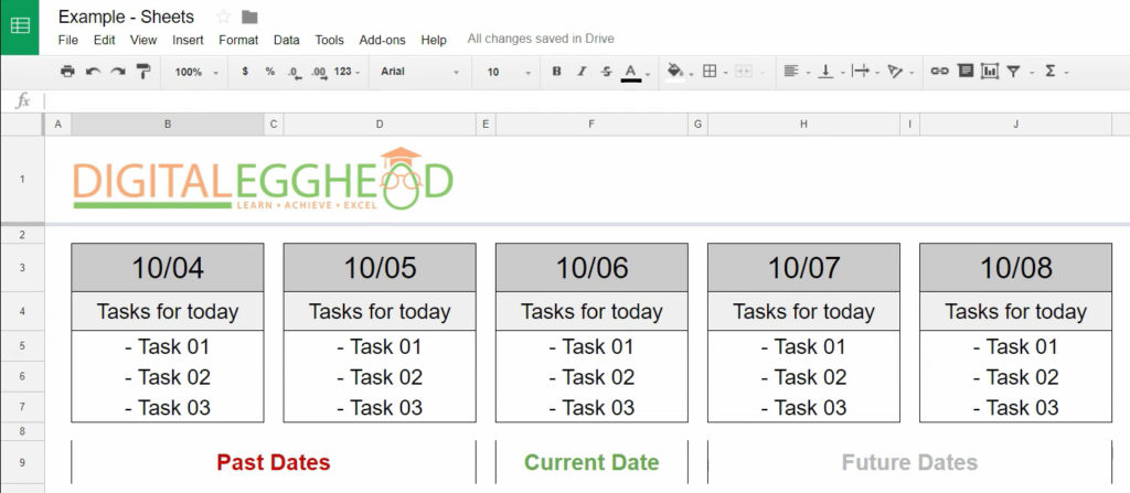
This is a relatively simple example, but you’ll be able to do a lot more with it once you see how it’s done.

Setting Up Conditional Date Formatting

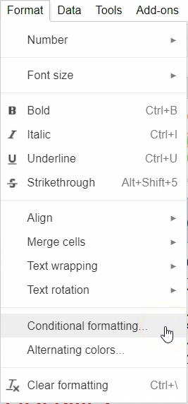
Start by highlighting the cells containing dates. Then click on “Format”, and “Conditional formatting”

This opens up a panel on the right side of the screen and immediately applies a default formatting to the cells.

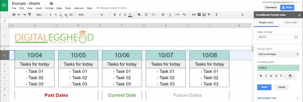
The default setting changes the cell to green if it is not empty. Set up the past date formatting first by clicking on the drop down for “Format cells if”

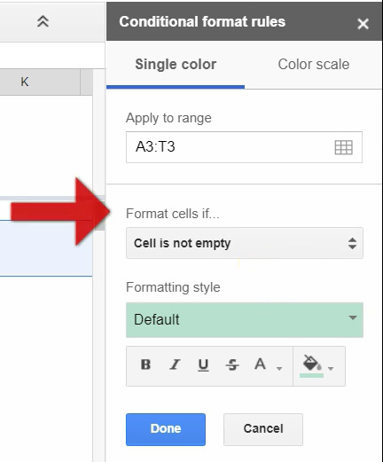
From the list, select “Date is before”

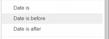
Another drop down link appears below the first one. By default, it has “Today” selected. You could also select any of the other options from the list, but today works for this example.

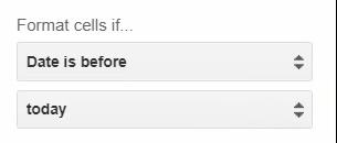
This will format the cell if it contains a date that is before the current date. Next, set up the format you want it to apply. You can change the green ‘default’ color to any color you want. You can also change the text color and format to something that works for your setup.

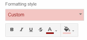
Now the cells that show the current day will display in the format that you set up. You can click on the “Add another rule” link at the bottom to set up different rules for other date requirements.

Example Conditional Date Formatting Setup

This example has formatting set up to show red for past dates, green for the current date, and gray for future dates.

 

That’s really all there is to this. You can do a lot more with it if you take some time to explore all of the options.

Watch the Video

Watch the video for conditional date formatting to see it in action.

I hope you found this article to be helpful. Comment below to and let me know what you think.

Learn more about Google’s amazing office apps with the Google Cloud Productivity course on Udemy.