Transpose Data In Google Sheets

Sometimes we end up with data in a column then later realize that it needs to be in a row, or vice versa. This is called transposing. Fortunately, Google Sheets makes it very easy to quickly transpose your data.

How to Transpose Data

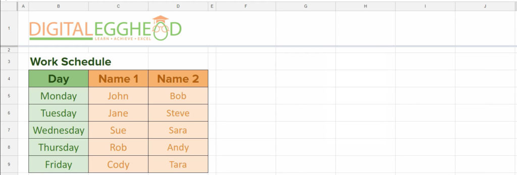
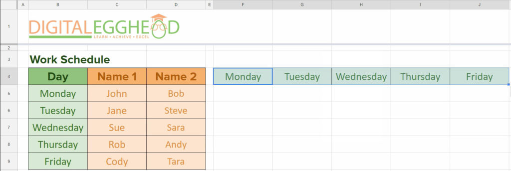
This example shows weekdays listed down one column, and names of people who are working on those days in the next two columns.

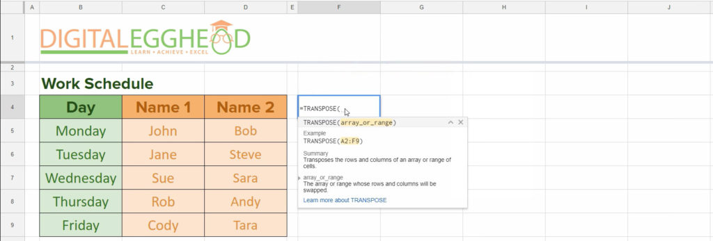
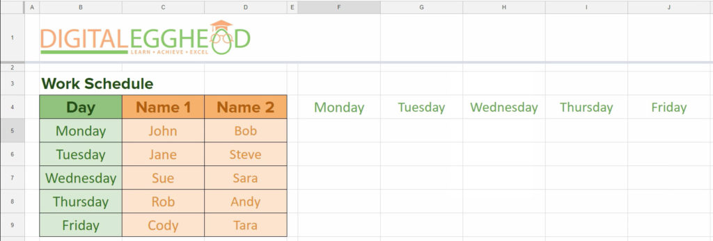
To change the weekdays from vertical to horizontal, select a blank cell and type in =TRANSPOSE.

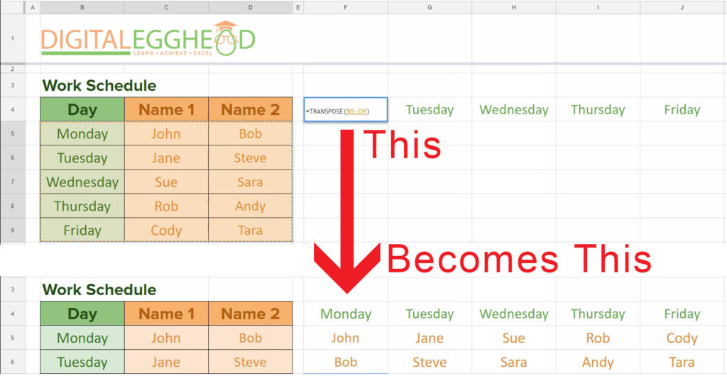
There is only one value for this function, which is the range of cells you want to transpose. Select the range and close the function. The data will instantly be listed across the row starting from the cell containing the function.

This can be done with as many cells as needed. You can simply select a bigger range that contains cells from additional columns.

This method works both ways for your data. If you use the function in another blank cell and select a row of data, it will be reversed, displaying the data down a column.

Another Way to Transpose

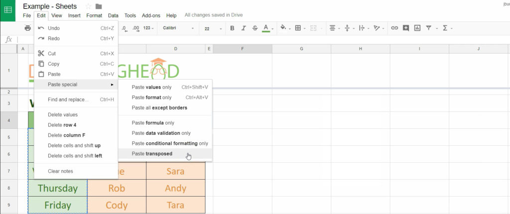
There is one more way to transpose, which is by using “Paste Special” Select a range of cells and copy it.

Then click on an empty cell, go to the Edit menu and select Paste Special > Paste Transposed

It will transpose all of the data with formatting applied.

And that’s it! It’s pretty easy to rearrange your data using Transpose in Google Sheets.

Watch the Video

Watch the transpose video to see it in action.

I hope you found this article to be helpful. Comment and let me know what you think.

Learn more about functions in Google Sheets with Udemy course, Understanding and Building Functions.

Click here to read more articles about Google Sheets and functions.